Next: Die Gateaux-Ableitung
Up: Die Frechet-Ableitung
Previous: Wichtige Eigenschaften der Frechet-Ableitung.
Contents
(I) Es sei  eine lineare stetige Abbildung zwischen
den normierten Räumen
eine lineare stetige Abbildung zwischen
den normierten Räumen  und
und  . Dann gilt für beliebiges

und damit
 für beliebiges
.
Die Frechet-Ableitung eines linearen stetigen Operators ist also dieser
Operator selbst.
für beliebiges
.
Die Frechet-Ableitung eines linearen stetigen Operators ist also dieser
Operator selbst.
Ist insbesondere
 und
und
 ,
so läßt sich die Abbildung
,
so läßt sich die Abbildung
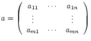
 durch eine Matrix
vom Typ  darstellen. Gleiches gilt dann für die Ableitung
 .
.
(II) Es sei
 und
und
 sowie
sowie
Für beliebiges
 und
und
 gilt
gilt
Damit gilt
 .
Wir werden uns später im Einzelnen mit der Berechnung von Frechet-Ableitungen
von Funktionen
.
Wir werden uns später im Einzelnen mit der Berechnung von Frechet-Ableitungen
von Funktionen
 beschäftigen.
(III) Es sei
![% latex2html id marker 30379
$ E=C^{1}([a,b],\mathbb{R}) $](img2279.png) und
und
![% latex2html id marker 30381
$ F=C([a,b],\mathbb{R}) $](img2280.png) mit
mit  . Wir betrachten die Abbildung
  gegeben
durch den Ausdruck
gegeben
durch den Ausdruck
welcher eine Kurzschreibweise für
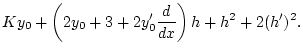
![$\displaystyle (Ky)(x)=(y(x))^{2}+3y(x)+2(y'(x))^{2},\quad x\in [a,b],$](img2283.png) |
(3.3.3.1) |
darstellt. Dabei verstehen wir
 und
und
 als rechtsseitige bzw. linksseitige Ableitung in den Randpunkten des
Intervalles.
als rechtsseitige bzw. linksseitige Ableitung in den Randpunkten des
Intervalles.
Die Abbildung  weist also jedem Punkt
  , d.h.
einer Funktion
, d.h.
einer Funktion
![% latex2html id marker 30401
$ y\in C^{1}([a,b],\mathbb{R}) $](img2286.png) , einen Bildpunkt
, einen Bildpunkt
 , d.h. eine Funktion
![% latex2html id marker 30405
$ Ky\in C([a,b],\mathbb{R}) $](img2288.png) zu. Bei der Berechnung der Frechet-Ableitung von im Punkt
zu. Bei der Berechnung der Frechet-Ableitung von im Punkt
 müssen wir die Funktion
![% latex2html id marker 30411
$ y_{0}\in C^{1}([a,b],\mathbb{R}) $](img2290.png) um ein Element
um ein Element  , d.h. eine Funktion
![% latex2html id marker 30415
$ h\in C^{1}([a,b],\mathbb{R}) $](img2291.png) verschieben. Dabei muß
verschieben. Dabei muß  klein bezüglich der
  -Norm
sein. Man erhält3.7
-Norm
sein. Man erhält3.7
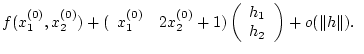
Wir stellen zunächst fest, daß
und damit
 für
für
 . Also gilt
 |
(3.3.3.2) |
wobei der Operator
 folgendermaßen wirkt
Dabei bildet er
folgendermaßen wirkt
Dabei bildet er
![% latex2html id marker 30469
$ E=C^{1}([a,b],\mathbb{R}) $](img2306.png) nach
nach
![% latex2html id marker 30471
$ F=C([a,b],\mathbb{R}) $](img2307.png) ab. Tatsächlich, aus
ab. Tatsächlich, aus
![% latex2html id marker 30473
$ y_{0},h\in C^{1}([a,b],\mathbb{R}) $](img2308.png) folgt
folgt
![% latex2html id marker 30475
$ y_{0},h,y_{0}^{\prime },h^{\prime }\in C([a,b],\mathbb{R}) $](img2309.png) und damit
und damit
![% latex2html id marker 30477
$ Th\in C([a,b],\mathbb{R}) $](img2310.png) . Desweiteren ist
. Desweiteren ist  offensichtlich linear im Argument . Es bleibt zu zeigen, daß
stetig von
offensichtlich linear im Argument . Es bleibt zu zeigen, daß
stetig von
![% latex2html id marker 30485
$ E=C^{1}([a,b],\mathbb{R}) $](img2311.png) nach
nach
![% latex2html id marker 30487
$ F=C([a,b],\mathbb{R}) $](img2312.png) wirkt. Dies folgt aus der Abschätzung
wirkt. Dies folgt aus der Abschätzung
mit
![% latex2html id marker 30510
$ C=\max \left\{ \Vert 2y_{0}+3\Vert _{C([a,b],\mathbb{R})},\Vert 2y_{0}^{\prime }\Vert _{C([a,b],\mathbb{R})}\right\} $](img2319.png) .
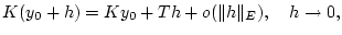
Aus der Darstellung (3.3.3.2) folgt nun,
daß
die Frechet-Ableitung der Abbildung im Punkt
.
Aus der Darstellung (3.3.3.2) folgt nun,
daß
die Frechet-Ableitung der Abbildung im Punkt  ist.
ist.
Aufgabe 3.3.3.1
Es sei
![% latex2html id marker 30524
$ E=C^{1}([a,b],\mathbb{R}) $](img2321.png)
und
![% latex2html id marker 30526
$ F=C([a,b],\mathbb{R}) $](img2322.png)
und man betrachte den Operator
gegeben
durch
wobei
und
als rechts -
und linksseitige Ableitungen in den Randpunkten zu verstehen sind.
Berechnen Sie die Frechet-Ableitung von

.
Aufgabe 3.3.3.2
Es sei
![% latex2html id marker 30544
$ E=C([a,b],\mathbb{R}) $](img2325.png)
und

. Wir
betrachten die Abbildung

gegeben durch
Berechnen Sie die Frechet-Ableitung von

.
Hinweis: Zeigen Sie in beiden Fällen, daß und lineare
stetige Operatoren zwischen den jeweiligen Räumen und
sind und verwenden Sie Beispiel (I).
Next: Die Gateaux-Ableitung
Up: Die Frechet-Ableitung
Previous: Wichtige Eigenschaften der Frechet-Ableitung.
Contents
2003-09-05
![$\displaystyle \left( \max _{x\in [a,b]}\left\vert h(x)\right\vert \right) ^{2}+2\left( \max _{x\in [a,b]}\left\vert h^{\prime }(x)\right\vert \right) ^{2}$](img2300.png)
![% latex2html id marker 30455
$\displaystyle 3\left( \max _{x\in [a,b]}\vert h(x...
...rt h^{\prime }(x)\vert\right) ^{2}=3\Vert h\Vert _{C^{1}([a,b],\mathbb{R})}^{2}$](img2301.png)
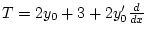
![% latex2html id marker 30512
$\displaystyle T=2y_{0}+3+2y_{0}^{\prime }\frac{d}{dx}\in \mathcal{L}\left( C^{1}([a,b],\mathbb{R}),C([a,b],\mathbb{R})\right) $](img2320.png)