Der Raum der stetigen linearen Operatoren.

Definition 3.2.5.1   Wir betrachten zwei normierte lineare Vektorräume $E$ und $F$ über $\mathbb{K}$. Mit $\mathcal{L}(E,F)$ bezeichnen wir die Menge der stetigen linearen Operatoren $T:D_{T}=E\to F$.

Für zwei gegebene Operatoren $T_{1},T_{2}\in \mathcal{L}(E,F)$ definieren wir deren Summe wiefolgt

$$(T_{1}+T_{2})x:=T_{1}x+T_{2}x,\quad x\in E.$$

Für $T\in \mathcal{L}(E,F)$ und $\alpha \in \mathbb{K}$ sei weiterhin $(\alpha \cdot T)$ der Operator

$$(\alpha \cdot T)x:=\alpha \cdot (Tx),\quad x\in E.$$

Die Abbildungen $T_{1}+T_{2}:E\to F$ ist dann linear, denn

$$(T_{1}+T_{2})(\alpha x+\beta y) = T_{1}(\alpha x+\beta y)+T_{2}(\alpha x+\beta y)$$

$$= \alpha T_{1}x+\beta T_{1}y+\alpha T_{2}x+\beta T_{2}y$$

$$= \alpha (T_{1}x+T_{2}x)+\beta (T_{1}y+T_{2}y)$$

$$= \alpha (T_{1}+T_{2})x+\beta (T_{1}+T_{2})y$$

für beliebige $\alpha ,\beta \in \mathbb{K}$ sowie $x,y\in E$.

Aufgabe 3.2.5.2   Zeigen Sie, daß $\alpha T:E\to F$ ebenfalls einen linearen Operator definiert.

Die Abbildung $T_{1}+T_{2}:E\to F$ ist stetig, denn als lineare stetige Operatoren sind $T_{1}$ und $T_{2}$ jeweils beschränkt, womit nach

$$\Vert (T_{1}+T_{2})x\Vert _{F} = \Vert T_{1}x+T_{2}x\Vert _{F}\leq \Vert T_{1}x\Vert _{F}+\Vert T_{2}x\Vert _{F}$$

$$\leq C_{1}\Vert x\Vert _{E}+C_{2}\Vert x\Vert _{E}=(C_{1}+C_{2})\Vert x\Vert _{E}$$

der lineare Operator $T_{1}+T_{2}$ auch beschränkt ist.

Aufgabe 3.2.5.3   Zeigen Sie, daß der Operator $\alpha T$ stetig ist.

Damit sind für $\mathcal{L}(E,F)$ die Operationen der Addition als auch der Multiplikation mit einem Skalar

$$+:\mathcal{L}(E,F)\times \mathcal{L... ...hcal{L}(E,F),\quad \cdot :\mathbb{K}\times \mathcal{L}(E,F)\to \mathcal{L}(E,F)$$

definiert.

Aufgabe 3.2.5.4   Zeigen Sie, daß die Menge $\mathcal{L}(E,F)$ mit den oben gegebenen Operationen $+$ und $\cdot$ die Struktur eines linearen Vektorraums besitzt. Das Nullelement $\mathbb{O}\in \mathcal{L}(E,F)$ ist dabei derjenige Operator, welcher alle Elemente $x\in E$ nach $0\in F$ abbildet.

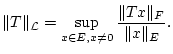
Definition 3.2.5.5   Für Operatoren $T\in \mathcal{L}(E,F)$ definieren wir die Größe

$$\Vert T\Vert _{\mathcal{L}}=\sup _{x\in E,x\neq 0}\frac{\Vert Tx\Vert _{F}}{\Vert x\Vert _{E}}.$$

Da alle Operatoren $T\in \mathcal{L}(E,F)$ beschränkt sind, so ist dies eine endliche Größe.

Aufgabe 3.2.5.6   Zeigen Sie, daß

$$\Vert T\Vert _{\mathcal{L}}=\sup _{... ...}=1}\Vert Tx\Vert _{F}=\sup _{x\in E:\Vert x\Vert _{E}\leq 1}\Vert Tx\Vert _{F}$$

sowie

$$\Vert Tx\Vert _{F}\leq \Vert T\Vert _{\mathcal{L}}\Vert x\Vert _{E},\quad x\in E.$$

Satz 3.2.5.7   Das Funktional $\Vert \cdot \Vert _{\mathcal{L}}$ definiert eine Norm auf dem Raum $\mathcal{L}(E,F)$.

$\blacktriangleright$ Wir verifizieren die Axiome der Norm. Wegen $\Vert Tx\Vert _{F}\geq 0$ und $\Vert x\Vert _{E}>0$ für $x\neq 0$ folgt $\Vert T\Vert _{\mathcal{L}}\geq 0$. Aus $\Vert T\Vert _{\mathcal{L}}=0$ folgt $\Vert Tx\Vert _{F}=0$ und somit $Tx=0$ für alle $x\in E$, d.h. $T=\mathbb{O}$.

Die Homogenität von $\Vert \cdot \Vert _{\mathcal{L}}$ folgt aus

$$\Vert \alpha T\Vert _{\mathcal{L}} = \sup _{x\in E:\Vert x\Vert _{E}=1}\Vert (\alpha T)x\Vert _{F}=\sup _{x\in E:\Vert x\Vert _{E}=1}\Vert \alpha (Tx)\Vert _{F}$$

$$= \sup _{x\in E:\Vert x\Vert _{E}=1}\vert\alpha \vert\Vert Tx\Vert _{F}=\vert\alpha \vert\Vert T\Vert _{\mathcal{L}}.$$

Zum Beweis der Dreiecksungleichung merken wir an, daß nach

$$\Vert T_{1}+T_{2}\Vert _{\mathcal{L}}=\sup _{x\in E:\Vert x\Vert _{E}=1}\Vert (T_{1}+T_{2})x\Vert _{F}$$

für jedes $\varepsilon >0$ ein solches $x_{\varepsilon }\in E$, $\Vert x_{\varepsilon }\Vert _{E}=1$ existiert, so daß

$$\Vert T_{1}+T_{2}\Vert _{\mathcal{L}}\leq \Vert (T_{1}+T_{2})x_{\varepsilon }\Vert _{F}+\varepsilon .$$

Dann gilt

$$\Vert T_{1}+T_{2}\Vert _{\mathcal{L}} \leq \Vert (T_{1}+T_{2})x_{\varepsilon }\Vert _{F}+\varepsilon =\Vert T_{1}x_{\varepsilon }+T_{2}x_{\varepsilon }\Vert _{F}+\varepsilon$$

$$\leq \Vert T_{1}x_{\varepsilon }\Vert _{F}+\Vert T_{2}x_{\varepsilon }\Vert _{F}+\varepsilon$$

$$\leq \sup _{x\in E:\Vert x\Vert _{E}=1}\Vert T_{1}x\Vert _{F}+\sup _{x\in E:\Vert x\Vert _{E}=1}\Vert T_{2}x\Vert _{F}+\varepsilon$$

$$= \Vert T_{1}\Vert _{\mathcal{L}}+\Vert T_{2}\Vert _{\mathcal{L}}+\varepsilon .$$

Im Grenzwert $\varepsilon \to 0+0$ folgt schließlich

$$\Vert T_{1}+T_{2}\Vert _{\mathcal{L}}\leq \Vert T_{1}\Vert _{\mathcal{L}}+\Vert T_{2}\Vert _{\mathcal{L}}.$$

$\blacktriangleleft$

Satz 3.2.5.8   Ist $F$ ein Banachraum, so ist $\left( \mathcal{L}(E,F),\Vert \cdot \Vert _{\mathcal{L}}\right)$ ebenfalls ein Banachraum.

$\blacktriangleright$ Wir müssen zeigen, daß jede Cauchy-Folge

$$\{T_{n}\}_{n\in \mathbb{N}}\in CF(\mathcal{L}(E,F))$$

gegen ein Element $T\in \mathcal{L}(E,F)$ konvergiert.

Schritt 1: Für die Cauchyfolge $\{T_{n}\}_{n\in \mathbb{N}}$ gilt

$$\forall _{\varepsilon >0}\exists _{... ..._{\varepsilon }}\parallel T_{n}-T_{m}\parallel _{\mathcal{L}}\leq \varepsilon .$$

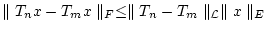Wegen $\parallel T_{n}x-T_{m}x\parallel _{F}\leq \parallel T_{n}-T_{m}\parallel _{\mathcal{L}}\parallel x\parallel _{E}$ folgt damit

$$\forall _{\varepsilon >0}\exists _{... ...parallel T_{n}x-T_{m}x\parallel _{F}\leq \varepsilon \parallel x\parallel _{E}.$$ (3.2.5.1)

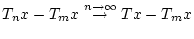
Also ist für jedes fixierte $x\in E$ die Folge $\{T_{n}x\}_{n\in \mathbb{N}}$ eine Cauchyfolge in $F$. Aufgrund der Vollständigkeit von $F$ existiert damit ein Grenzwert

$$t_{x}=\lim _{n\to \infty }T_{n}x\in F$$$$\quad \mbox {für\, jedes}\quad x\in E.$$

Schritt 2: Wir betrachten die Abbildung $T:E\to F$ gegeben durch

$$Tx=t_{x}=\lim _{n\to \infty }T_{n}x,\quad x\in E.$$

Wir zeigen, daß $T$ ein linearer Operator ist. Tatsächlich, für $x,y\in E$ und $\alpha ,\beta \in \mathbb{K}$ gilt

$$T(\alpha x+\beta y) = t_{\alpha x+\beta y}=\lim _{n\to \infty }T_{n}(\alpha x+\beta y)=\lim _{n\to \infty }(\alpha T_{n}x+\beta T_{n}y)$$

$$= \lim _{n\to \infty }\alpha T_{n}x+\lim _{n\to \infty }\beta T_{n}y=\alpha t_{x}+\beta t_{y}=\alpha Tx+\beta Ty.$$

Schritt 3: Wir zeigen nun, daß die lineare Abbildung $T$ beschränkt und damit stetig ist. Dazu merken wir zunächst an, daß die Cauchyfolge $\{T_{n}\}_{n\in \mathbb{N}}$ in $\mathcal{L}(E,F)$ beschränkt ist, d.h.

$$\parallel T_{n}\parallel _{\mathcal{L}}\leq C,\quad n\in \mathbb{N},$$

für ein geeignetes $C<\infty$. Aus der Stetigkeit der Norm $\parallel \cdot \parallel _{F}$ folgt dann

$$\parallel Tx\parallel _{F} = \parallel \lim _{n\to \infty }T_{n}x\parallel _{F}=\lim _{n\to \infty }\parallel T_{n}x\parallel _{F}$$

$$\leq \limsup _{n\to \infty }\parallel T_... ...parallel _{\mathcal{L}}\parallel x\parallel _{E}\leq C\parallel x\parallel _{E}$$

für beliebiges $x\in E$.

Schritt 4: Aus den letzten beiden Schritten folgt $T\in \mathcal{L}(E,F)$. Es bleibt zu zeigen, daß $\{T_{n}\}_{n\in \mathbb{N}}$ in $\mathcal{L}(E,F)$ gegen $T$ konvergiert. Dazu gehen wir in (3.2.5.1) für $m\geq N_{\varepsilon }$ zum Grenzwert $n\to \infty$ über, woraus man unter der Berücksichtigung der Stetigkeit von $\Vert \cdot \Vert _{F}$ wegen $T_{n}x-T_{m}x\stackrel{n\to \infty }{\to }Tx-T_{m}x$ die Beziehung

$$\Vert (T-T_{m})x\Vert _{F} = \Vert Tx-T_{m}x\Vert _{F}=\lim _{n\to \infty }\Vert T_{n}x-T_{m}x\Vert _{F}$$

$$\leq \varepsilon \Vert x\Vert _{E} \quad \mbox {für\, beliebiges}\quad x\in E$$

erhält. Dies impliziert

$$\Vert T-T_{m}\Vert _{\mathcal{L}(E,F)}\leq \varepsilon$$$$\quad \mbox {für}\quad m\geq N_{\varepsilon }$$

und damit $T_{n}\stackrel{\mathcal{L}(E,F)}{\to }T$. $\blacktriangleleft$