Detailed Description

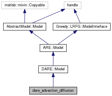
Implicit Euler discretization of a finite-difference convection-diffusion model.

This model is constructed in such a way, that it can follow a given trajectory - or at least it tries to follow it. Use the SIMULATE function to simulate!

Andreas Schmidt, 2016

Definition at line 17 of file dare_advection_diffusion.m.

Inheritance diagram for dare_advection_diffusion:

[legend]

Collaboration diagram for dare_advection_diffusion:

[legend]

Public Member Functions
	dare_advection_diffusion (n)

function r =	E_comp ()

function r =	E_coeff ()

function r =	A_comp ()

function r =	A_coeff ()

function r =	B_comp ()

function r =	B_coeff ()

function r =	C ()

function r =	C_comp ()

function r =	C_coeff ()

function r =	R_coeff ()

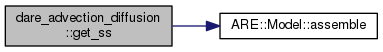
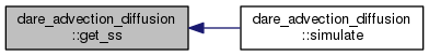
function s =	get_ss (model_data, dsim)
	GET_SS Get the state space model for simulation purpose If dsim is provided, a closed-loop simulation is performed. More...

function [ t , y , u , r , x ] =	simulate (model_data, T, r, sim, x0)
	SIMULATE - Simulate the system for a given time T ...... final time r ...... reference value or vector sim .... simulation used for feedback. More...

Public Member Functions inherited from DARE.Model
function pt =	problem_type ()

function g =	gamma (ModelData model_data, dsim)

function n =	closed_loop_norm (ModelData model_data, dsim)
	CLOSED_LOOP_NORM Implementation of an efficient algorithm for the approximation of the 2-norm of the closed-loop matrix. More...

function [ stable , cleig ] =	closed_loop_stable (ModelData model_data, dsim)
	CLOSED_LOOP_STABLE Implementation of an efficient algorithm for checking whether the closed loop matrix gives a stable system. This is done by calculting the maximum eigenvalue of the closed loop system. More...

Public Member Functions inherited from ARE.Model
virtual function [ A , A , B ] =	B_comp (ModelData model_data, this,ModelData model_data)

function [ E , A , B , C , Q , R ] =	assemble (md)
	ASSEMBLE Assembles all the data matrices. This function works for both, the reduced and the full model. More...

function E =	mass_matrix (md)
	MASS_MATRIX Get the mass matrix of the problem This function is used by the LRFG algorithm for the orthogonalization procedure. More...

function g =	gamma (ModelData model_data, dsim)
	GAMMA Calculate the value of gamma. This is used by applying the Lyapunov equation method. More...

function R =	R_coeff ()

function Q =	Q_coeff ()

function E =	E_coeff ()

function C =	C_coeff ()

function B =	B_coeff ()

function R =	R_comp (ModelData model_data)

function Q =	Q_comp (ModelData model_data)

function E =	E_comp (ModelData model_data)

function C =	C_comp (ModelData model_data)

function [ T , y , x ] =	simulate (ModelData model_data, dsim)
	SIMULATE This function simulates the underlying LTI model If you provide dsim, the closed-loop simulation will be performed. More...

Public Member Functions inherited from AbstractModel.Model
virtual function dsim =	detailed_simulation (ModelData model_data)
	DETAILED_SIMULATION The function DETAILED_SIMULATION returns an instance of SimData and. More...

virtual function rsim =	rb_simulation (IReducedData reduced_data)
	REDUCED_SIMULATION This function should return a reduced simulation of type RBSimData. More...

function ModelData model_data =	gen_model_data ()
	GEN_MODEL_DATA Use this function in order to create a class of type ModelData which contains all the large-scale model data such as the discretized operators. More...

function IDetailedData detailed_data =	gen_detailed_data (ModelData model_data)
	GEN_DETAILED_DATA Call the basis generation algorithm. More...

function IReducedData reduced_data =	gen_reduced_data (IDetailedData detailed_data)
	GEN_REDUCED_DATA Get the reduced data structures. More...

function pt =	problem_type ()
	PROBLEM_TYPE Use this function to determine the problem type. So consider overwriting it if necessary! TODO: implement a smart interface that automatically generates the correct. More...

function mu =	get_mu ()
	Get the parameter values. More...

function this =	set_mu (mu)
	Set the parameter values. More...

Public Attributes
	mu = "[1 1 3]"

	mu_names = {"'mu_diffusion', 'mu_adv_y', 'lambda_tracking'"}

	mu_ranges = {" [0.1, 2], [0,10], [1, 10]"}

	n0

	dt = 0.05

Public Attributes inherited from DARE.Model
	RB_closed_loop_norm = "fro"

	RB_closed_loop_stable = false

Public Attributes inherited from ARE.Model
	enable_error_estimator = false

	calc_residual = true

	RB_gamma_mode = "Kernel"
	Additional fields for basis generation: More...

	RB_gamma_enabled = 1

	RB_gamma_settings = {""}

	p
	The number of measurement outputs.

	m
	The number of control inputs and measurements.

	n

	model_data

Public Attributes inherited from AbstractModel.Model
	mu

	mu_names

	mu_ranges

Public Attributes inherited from Greedy.LRFG.ModelInterface
	RB_greedy_tolerance = 1e-4

	RB_orthonormalize_E = true

	RB_error_indicator = "residual"

	RB_pod_tolerance = 0.99

	RB_pod_max_extension = 10

	RB_M_train = "Uniform"

Protected Member Functions
function [ A , name ] =	my_2d_matrix (n0, fx_str, fy_str, g_str, mu_str)

function v =	my_2d_vector (n0, f_str)

Member Function Documentation

function s = dare_advection_diffusion.get_ss	(	model_data,
		dsim
	)

GET_SS Get the state space model for simulation purpose If dsim is provided, a closed-loop simulation is performed.

Parameters

model_data	model data
dsim	dsim

Return values

s s

Definition at line 113 of file dare_advection_diffusion.m.

Here is the call graph for this function:

Here is the caller graph for this function:

function [ t , y , u , r , x ] = dare_advection_diffusion.simulate	(	model_data,
		T,
		r,
		sim,
		x0
	)

SIMULATE - Simulate the system for a given time T ...... final time r ...... reference value or vector sim .... simulation used for feedback.

This function returns the following vectors: t ....... time span for simulation y ....... output value u ....... control signal r ....... the reference signal x .......

Parameters

model_data	model data
T	T
r	r
sim	sim
x0	x0

Return values

t	t
y	y
u	u
r	r
x	x

Definition at line 142 of file dare_advection_diffusion.m.

Here is the call graph for this function:

The documentation for this class was generated from the following file:

models/dare_advection_diffusion.m

Detailed Description

Public Member Functions

Public Attributes

Protected Member Functions

Member Function Documentation