Wir wollen den in der Wiederholung mit III bezeichneten Lösungsweg verwenden.
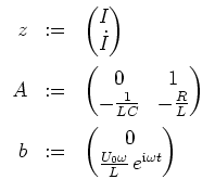
Wir setzen hierzu
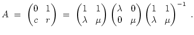
Wir wollen
![]() berechnen. Da die Matrix
berechnen. Da die Matrix
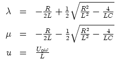
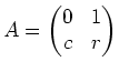 Parameter enthält, gehen wir näher auf diese Berechnung ein. Ihre Eigenwerte sind
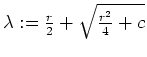 und
und
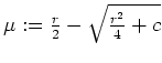 , und nach Voraussetzung an
![]() verschieden und beide reell.
verschieden und beide reell.
Die Jordanform ergibt sich zu
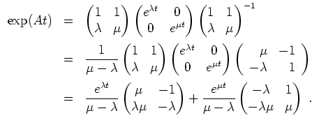
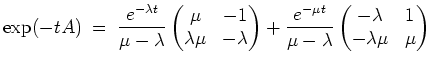
Für die Variation der Konstanten beachten wir zunächst, daß wir nach Ersetzen von
![]() durch
durch
![]()
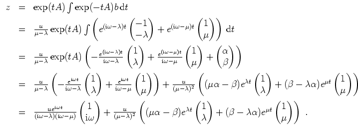
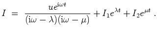
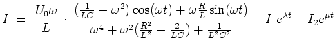
 liefert die allgemeine Lösung

Skizze für
![]() ,
,
![]() ,
,
![]() ,
,
![]() ,
,
![]() (von oben nach unten),
(von oben nach unten),
![]() und
und
![]() .
.
![\includegraphics[width = 8cm]{RCL.eps}](img40.png)
Interpretation. Nach Abklingen des homogenen Bestandteils
![]() verbleibt für große
verbleibt für große
![]() eine Schwingung mit Frequenz
eine Schwingung mit Frequenz
![]() gleich der Erregerfrequenz.
Die Phasenverschiebung im Vergleich zur Erregerspannung, sowie die Amplitude können der oben hergeleiteten Formel entnommen werden.
gleich der Erregerfrequenz.
Die Phasenverschiebung im Vergleich zur Erregerspannung, sowie die Amplitude können der oben hergeleiteten Formel entnommen werden.